The pathway to finding a solution or outcome to such an open and abstract project is still very much in flux. The examples below are one possible offshoot of a previous experiment. These are a couple of weeks old now, so the methodology behind a solution has developed and evolved since, but nonetheless, they are worth posting in an attempt to find a footing.
The initial ideas spawned from flattening curves and then extruding them against one another, or revolving them within a three dimensional space. Already, some of these have some interesting decisions. Some are very formal, with structure and weight, whilst others hover in negative space and demonstrate options for manufacture.
These options are far more in line with the aesthetic and ideas of traditional sculpture. In my role, I'm trying to find some alternative paths. These are not outcomes in any way, but demonstrate the breaking of traditional approach, attempting to create forms that sit in alternative spaces or that simply break from traditional ideas that we may have had.
In many ways these are just bizarre experiments in an attempt to find some interesting pathway through the project. But these ideas are already a few weeks old and new thoughts / research are being discussed, so keep updated for some new methodologies in the next few weeks.
Another sculpture to add to the collection. This time I thought I would
post without the 'how', and just see what the response is:
Conductor's Arm - Taken from Part 1 - Requiem
I've been thinking more about how these sculptures could be represented
physically. While I'm not saying this example is structurally sound
(there are still some free floating shapes!), I hope it communicates how
something like this could be constructed.
The colours are arbitrary, but for future examples, I think that this is something that could come from the mood of the music.
Continuing with my experimentations; I wanted to find an effective solution to shrink wrap a mesh around the curves. I also wanted to explore ways in which to scan the 3D curve data (like an MRI scan) to build up a series of flat sections of the curve.
All curves and sculptures are from part 3 of Verdi's Requiem, 'Offertorio'.
With the help of some plug-ins I was able to create this structure.
The idea here is that we could create a wire frame structure which we can shrink wrap some kind of material around, to create a light translucent sculpture. If only we could reconstruct one of the original 3D curves for real, I think the translucent effect would look quite good with the silhouette of the curve inside. Or at least with something inside.
The same technique was applied to this sculpture.
It is similar but different as I didn't shrink wrap around the original curve. Instead I traced sections of the curve from two sides at various depths. I did this by creating a camera with a tiny clipping distance to run through the curve from a particular angle. This allows me to scan through the curve and get a picture of a slice of the curve. I traced around whatever I saw in the view by hand. The resulting curves were then used for wrapping a mesh around in the same way as above.
Since the above image is a bit difficult to interpret, the following image just shows four of the traced curves from the front view at different depths.
Interestingly enough, watching the camera/scanner run through the curve produces it's own interesting animation!
So how did I shrink wrap the mesh around the curves? A dense spherical mesh was created as a starting point. The mesh was then snapped 'magnetically' to the curve with the help of a freely downloadable plug-in called prAttractNode, which I found on Creative Crash. I maximised the falloff so that the whole mesh was attracted to the shape of the curve. This is the resulting mesh.
The plug-in has options for creating a smoother look, but the results were not satisfying so I kept the hard edge look and decided to rely on something else to smooth the mesh out. I achieved this with another plug-in (which I wrote myself several months back) specifically designed for smoothing high poly meshes. Here you can see the effect it has on the mesh.
Using the two plug-ins in combination works well to create various shapes influenced by the curve. Because they are deformer nodes, it means that the effect is animatable too. For example, by changing the size of the source shape, you can create shapes that wriggle through the curve.
It looks quite good when you put a series of flat sheets into the structure.
Already, this project has overcome the unenviable task of creating form from data, embarking on the task of creating art from numbers or mathematics. These technical challenges were intense and complex, far too complex for myself, and the work that Alan and Ethan have undertaken has been quite astounding. A real headache destroyed with some superbly clever scripting and scene setup. And from this, from these csv files, a set of curves have been born that directly translate to the creation of Requiem. From movement to music, data to sculpture, it is a project that seems so pure in its representation. Something so different from my usual practise. I will be writing more about some of this conceptual stuff soon, but my job now is to join the team as a artsy fartsy experimenter. I've stayed clear of the technical setup (not only because my brain lacks that capacity) because I wanted to approach from the outside, purely to experiment with the tools and setup created. Already, I've had some fascinating results, and I can see plenty more in the future. So, here is the first contact sheet for Requiem by myself.
The future of the project is still wonderfully open, with ideas and conclusions born from the act of creation. I'll be experimenting plenty more with different approaches and data sets, but for now, this demonstrates some initial creation from data. I'll also discuss how some of these were made, but for now, I'd like to keep the experimentation free from technical details. So, I guess, more soon.
After further experimentation with the curves, I have come up with another technique. It's completely procedural, and is animated so that you can see what the shape looks like over time. Here it is.
This effect is made possible with the detachCurve node in Maya. This is called the Detach Curves command in the Edit Curves menu. It is capable of cutting a curve into smaller sections. You need to specify the points along the curve before using it. By default it will create the new curves and delete the original, however by going into the commands options you can chose to 'keep original', which will leave the original curve unchanged and generate new curves with a connection to the original. With the detachCurve Node that is created, you can animate the points at which the curves are cut from, allowing you to create an animated curve, which follows the path of the original.
It is similar to how a motion path works, except rather than tracing a single point along the curve, you can trace a portion of the curve. As I said, it is completely procedural, meaning that the original curve can still be modified and the traced curve will update to any changes.
To create the final structure, I lofted between two copies of the traced curve, one of which was flattened, while the other remained 3D. Hopefully this video from a top down view shows what's going on.
The green line follows the path of the blue line, and the white line is the flattened curve.
Now we have the data available in Maya (as both animation and nurbs curves), the next step is to derive as many interesting shapes and designs from it as possible. I have been able to come up with a few techniques.
The following technique offers a way to potentially generate an infinite number of shapes from the curve data. Looking at just one of the many 3D curves we have can reveal many different shapes within the intersecting lines, however depending on the angle you look from, it will appear different, and dramatically change the look of the curves and shapes within.
The screen shot below shows the same curve from three different angles, clearly demonstrating this effect.
By placing one of these curves into a group and scaling the group down in one axis, we can generate a flattened curve, representing what the curve would look like from that angle. By rotating the curve from within the group we can quickly preview the flattened curve from any angle.
The trick is how can we quickly break the curve into individual pieces at every point the lines intersect. Once we can do that we can build the individual shapes.
If we do a surface planer operation on the flattened curve, it will fill in the entire shape with a flat surface.
We can then go into the Trim Edge mode for nurbs surfaces, where we can then select different intersecting lines to extract the individual curve pieces. We use Duplicate Surface Curves in the Edit Curves menu to do this. We could select all the lines at once and get every piece of curve or just select the ones we need.
Either way, once we have the curve pieces extracted we can select whatever we need to make a shape and use the surface planer operation to build it.
From here we can convert to polygons and extrude it and do whatever else we can think of.
If we were to gather enough of these abstract shapes, we can use them to create more complex sculptures.
Here are a few more ideas.
A more straight forward interpretation of one of the 3D curves is to simply extrude a shape along its path. In this example I extruded several smaller shapes to create a brush stroke look. I suppose we could use the shapes generated from curves with the technique I explained above.
I created this coloured version, by using the samplerInfo node to sample the world space location (i.e. x,y,z became the new r,g,b values) and finished off with some colour remapping.
In this one, I wrote a quick script to duplicate the profile shape along the path and adjusted it's scale based on another piece of animation data. By lofting the duplicated profile curves in the correct order, we can create a shape that follows the path while also varying the width of the path at the same time. After the extra effort to get something more interesting I don't think it notices that much!
And here's a coloured version, same as the last example.
Since I haven't posted the following anywhere else yet, I will also include this experiment.
This was achieved before we even had the final .csv script, and shows what can be done with a particle simulation. In the following example I attach a particle emitter to one of the pieces of animation data, to trace the path with particles. I then generated a blobby mesh, which gets smoothed/averaged to clean up the shape. The particles die after a set period of time so as you play through the simulation, you're viewing a segment of the data as time goes on.
While I've only shown a few examples in this post (it's been more focused on techniques), I think they are good starting points to generate more designs!
After clipping and aligning the data to find the ‘true
concert’ the next stage was to cut the performance in to manageable sections so
that each generated curve would be more musically and visually specific. Each
section of the seven chosen represents a natural break in the music, these are:
1: Requiem
2: Dies Irae
3: Offertorio
4: Sanctusi
5: Agnus Dei
6: Lux Aterna
7: Libera Me
To achieve this in Maya the timeline was adjusted (using
a little math) to pinpoint the frames representing the breaks, fine tuning by
ear was also needed to nuance the start and end of the break. Using the new time codes curves were generated for each data stream, shown below.
After Ethan’s great work with Python scripting to allow the
.csv data to be turned in to animation streams and spline curves in Maya we faced the
next two new challenges;
Challenge 1 - Finding
True Time: Although the ‘ecs_CsvToMaya.py’ script allowed the data into Maya it
had no multiplication factor to make it match ‘true time’. In essence over two hours of data was being compressed in to fifty frames (two seconds).
Challenge 2– Different
lengths of Data: Each data file (.csv) ,Choir Heart Rate, Conductors Feet
Movement, etc had a different length (recording time) due to the complexities
of setting up devices whilst on location. The Cellist for example was recorded
for over two hours but the performance only lasts for one and half hours. This meant
that each data stream needed to be aligned and then ‘top and tailed’ to find
the concert performance.
Solution - The
solution for both problems relied upon finding an anchor point to match each
stream. Alongside each
data stream we also recorded sepereate audio/video files as reference which meant that we were able
to 'stack & achor' each on a timeline in Premiere. To do this we used the end of the performance
(last notes) to identify a consistant ‘time based clipping guide’. For example,
Aligned Audio /
Visual in Premiere
Choir
File Length: 2hrs 15m
27s - Concert Start Time at: 40m 12s - Concert End Time at: 2hrs 5mins 04s
Conductor
File Length: 2hrs 00m
08s - Concert Start Time at: 26m 24s - Concert End Time at: 1hrs 51mins 28s
Cellist
File Length: 2hrs 09m
29s - Concert Start Time at: 30m 19s - Concert End Time at: 1hrs 55mins 25s
ZDepth
File Length: 1hrs 25m
39s - Concert Start Time 7s - Concert End Time at: 1hrs 24mins 49s
Once we had this information we were able to
calculate that the multiplication factor to unlock true time (per file),
was a factor of ‘2.4’. Once this was added to the script we could be
sure that anything created in Maya would be a true visual representation of time
vs data. Finally, by using the ‘start/end time of the concert’ and Maya’s
timeline we were then able to set the time range to the concert only ensuring that each curve or animation generate was clipped to the correct length (‘ecs_CsvToMaya.py’uses the range of the timeline to calculate).
Cellist Arm Data
Stream Created Clipped in Maya
Success! - The next step, chopping the concert into sections…
As anyone whose following this blog knows, we have a collection of files containing data that was captured at a performance of Verdi's 'Requiem', using various sensors connected to several participants. The purpose of capturing this data was so that we could use it to create something in 3D that derives from that performance.
The files in question contain Comma Separated Values, simply known as .csv files. Since Autodesk Maya cannot read these files and no obvious solution (script/plug-in) could be found on the internet, it would seem like an impossible task to be able to make use of them in any meaningful way, but it's not 'game over' just yet!
My brief was to use the Python programming language to bridge the gap between the files and Maya. I would need to find a way to read the files, interpret the data and then find ways to represent that data in Maya.
In this post I will be outlining my progress on the script, covering my research and thinking behind it, and finishing with an overview of how it works and how to use it.
The CSV File
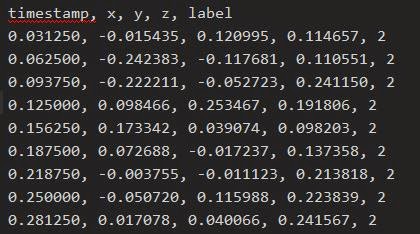
The first thing to understand about the .csv file type is that there are no strict rules on the format of the file; only that it is written in plain text (so it is humanly readable if opened in a text editor), that each line is a record containing fields separated by a delimiter (usually a comma), and that each line contains the same sequence of fields. While there are no requirements to label the fields, it is also common to use the first line to contain headings for each field. In our case all the .csv files we have use headings on the first line. Here is one of our examples:
What the Script Does
The script does several things:
The first function of the script is specifically for reading the data from any given file.
getCsvData("Path/to/a/file.csv")
This takes a file path, reads a file and it then returns a Python object containing the data in a format that can easily be used by other Python functions. It does this by reading the file line by line, using the commas to split each line of text into their individual values.
It assumes the first line contains the headings, so it will use that information to create a Python Dictionary Object, using each heading to contain a list for its values. As the script continues to read each line, the values are appended to the corresponding list in the dictionary. It is this dictionary object that is then returned by this function. Here is an example of what a Python dictionary looks like:
Each dictionary entry is a key:value pair. 'timestamp' being the key to access a Python List (the square brackets). The list would look something like this:
['0.031250', '0.062500', '0.093750', '0.125000']
Once a file has been read by this function and its output stored in a variable, it is possible to use the data within Python without needing to re-read the file.
As said previously, .csv files can contain any kind of data, some of which is not necessarily going to be useful to Maya. While the above function is designed to read any .csv file into Python, what we do next with this data is going to be specific for each file.
The next few functions written for the script are written specifically for the files that we are working with.
I shall use the heart rate file as an example of how I use the data.
This function creates an empty group node in Maya with the following animated attributes.
speed pace heartRate averageSpeed averagePace averageHeartRate latitude longitude distance
This .csv data contains a "Workout Time (secs)" column. The function accesses the values in that column, (in this case, the current time in seconds), and for each one, the corresponding attribute values are accessed and a key frame is set at that time, and that value.
The script also uses a helper function to convert the time from seconds to frames, taking the scene frame rate into account automatically. Here is what the extracted animation data looks like:
Writing a function to read the csv data object is fairy straight forward as shown in this Python code snippet.
def printCsvColumn(csvData, columnName)

    for i in range(len(csvData[columnName])):
        print csvData[columnName][i]
This code takes a csvData object and the name of a column, and prints out the values of that column.
Basic Usage of the Script
For all team mates on project Requiem, here is a quick overview on how to use the script.
To install the script you need to put the .py file inside one of the 3 script folders in your local maya settings folder. As an example:
Windows: <drive>:\Documents and Settings\<username>\My Documents\maya\<Version>\scripts
Mac OS X: ~/Library/Preferences/Autodesk/maya/<version>/scripts
Linux: ~/maya/<version>/scripts
Once this is done, run Maya and open up the script editor. Then inside a Python tab, run the following:
First we need to 'import' the script's functions. We use the namespace of 'csv' so we don't have to type out the full name.
import ecs_CsvToMaya as csv
Next we run the function 'getCsvData' and parse in the file path to a csv file as a string. The data is returned and stored in the variable 'csvData':
csvData = csv.getCsvData("Path/to/a/file.csv")
Note the quotation marks around the string, and the 'csv.' before the function name. If we didn't use the namespace when importing the module, we would have to write it like this:
ecs_CsvToMaya.getCsvData("Path/to/a/file.csv")
Now that we have the data available in Python we can use the other functions in the script to represent that data as keyframes. As each file is different we need to make sure we use the right function for the right file.
For the heart rate file, we need to use this function:
csv.createCsvHeartRateData(csvData)
This will create an empty group with all the relevant data animated on some custom attributes.
However for the rest of the files we can use this function:
csv.createCsvSensorData(csvData)
This will create a locator with the translate X, Y, and Z attributes animated.
So the completed code to run in Maya should look something like this:
So for each file we need to read in the data, then use the correct function to get the data into Maya.
In this case the heart rate file is the only exception, and for the rest we can use the other function.
On last set of functions have also been included, that generate Nurbs Curves from the animation data.
To use these you can run either of the following commands in Python (replacing with correct node and attribute names):
You can use the Maya time slider to select a time range from which to generate the curve from.
create3DCurve() specifically works on the translate X, Y and Z attributes to generate a full 3D curve, while the create2DCurve() will generate a flat curve on any other attribute. Here is an example of what the 'pace' attribute generated from the heart rate file:
Taking the Script Further
Currently the script will not be made publicly available, as the script is very much geared towards this project only. However it is my intention to continue developing this script so that it can be used on other projects, and by other people. I'm thinking that the tool would need to be generalised so that it could be possible to analyse any csv file from within Maya and choose how to interpret the data, rather than needing to write specific functions on a per-file basis.
Perhaps it would be possible to provide a set of nodes that are designed to interpret the data in different ways, which could then be plugged into existing Maya nodes to animate objects, create effects or generate meshes on the fly etc; and of course, some kind of graphical user interface.
So there we have it! I hope that readers have found it interesting, and informative.